STWO Prover Analysis

Composition Polynomial

  • Before running the FRI protocol, we compute the composition polynomial
  • It combines all constraint polynomials with powers of a challenge
\textcolor{lightgreen}{\textsf{CP}(X)} = \sum_{i=1}^{n} \textcolor{orange}{\alpha^{i}} \cdot \frac{\textcolor{red}{f_i(X)}}{Z(X)}
  • All constraint polynomials \(\textcolor{red}{f_1(X), \dots, f_n(X)}\) evaluate to \(0\) on trace domain
  • Currently, \(\texttt{compute\_composition\_polynomial}\) takes \(\approx 50\%\) of the prover time
  • Need to understand the function and its data flow to speed it up

\(\texttt{compute\_composition\_polynomial}\)

\(\textsf{trace}\)

\(\alpha\)

\(\textsf{CP}(X)\)

Trace Structure

Component A

Component B

Preprocessing trace

\underbrace{\hspace{1.1cm}}

Execution trace

\underbrace{\hspace{19.5cm}}

Interaction trace

\underbrace{\hspace{6.9cm}}

Trace Structure

Component A

Component B

\textsf{CP}_A(X)
\textsf{CP}_B(X)
\textsf{CP}(X)
\textsf{acc}

Trace domain size

2^{t_1}
2^{e_1}

Eval domain size

n_1

No of constraints

Trace domain size

2^{t_2}
2^{e_2}

Eval domain size

n_2

No of constraints

\(\texttt{compute\_composition\_polynomial}\)

\textsf{trace}
\alpha
\textsf{C}_1
\begin{bmatrix} \\ \textsf{CP} \\ \\ \end{bmatrix}_{2^{E} \times 1}
\textsf{pow}
\left[\alpha^0, \alpha^1, \dots, \alpha^{M-1}\right]
\begin{bmatrix} \\ \textsf{CP}^{(C)} \\ \\ \end{bmatrix}_{2^e \times 1}
\textsf{eval}
\begin{bmatrix} \\ \ \Lambda^{(C)}(\ \textsf{trace} \ ) \ \\ \\ \end{bmatrix}_{2^e \times n_C}
\text{s.t. }\Lambda^{(C)} = \{ \lambda_1, \dots, \lambda_{n_C} \}
\textsf{CP}(X) = \frac{\sum_{i=1}^{n} \alpha^{i} \cdot f_i(X)}{Z(X)}
|E| = 2^e \ge |T| = 2^t
\textsf{vanish}
\left[Z(\omega_1), \dots, Z(\omega_{2^{e-t}})\right]
\textsf{binv}
\left[Z^{-1}(\omega_1), ..., Z^{-1}(\omega_{2^{e-t}})\right]
n_c \textsf{ challenges}
\textsf{acc}
\begin{bmatrix} \\ \textsf{num}^{(C)} \\ \\ \end{bmatrix}_{2^e \times 1}
\textsf{mul}
\begin{bmatrix} \\ \textsf{CP}^{(K)} \\ \\ \end{bmatrix}_{2^{e_k} \times 1}
\begin{bmatrix} \\ \textsf{CP}^{(1)} \\ \\ \end{bmatrix}_{2^{e_1} \times 1}
\begin{bmatrix} \\ \textsf{CP}^{(2)} \\ \\ \end{bmatrix}_{2^{e_2} \times 1}
\vdots
\vdots
\textsf{final}

Memory Considerations

Component Eval domain Total columns # constraints Max Memory (MB)
Scheduler 2^17 409 6 68
Round 1 2^20 645 129 1074
Round 2 2^18 645 129 269
Xor 12 2^17 772 128 135
Xor 9 2^15 52 8 3
Xor 8 2^13 52 8 0.3
Xor 7 2^11 52 8 0.15
Xor 4 2^9 9 8 0.01
Full trace 2^20 2636 424 4300

Example: \(2^{16}\) instances of Blake2s hash

Implementation Steps

  • Extend polynomial API for DCCT (necessary for circle STARKs)
  • Batch inversion for vanishing polynomial (optional?)
    • Pre-compute and cache vanishing polynomial inversions?
  • Construct a kernel using polynomial API to process one component
  • Run different components on independent streams
  • Construct a kernel to compute the final composition polynomial
  • Polynomial API currently only uses one stream (multi-stream polyAPI?)

Timeline and Man-hours

With polynomial API Without polynomial API
Easier to write Harder but more control
Requires DCCT in polyAPI and
batch inversion
Can require batch inversion
Preparation: 3 days Preparation: 1-2 days
Can use only one stream Multi-stream for components
Could be slower (single stream) Should be faster with multiple streams
Implementation: 2 days Implementation: 3 days

FRI Quotient

Component A

Component B

Preprocessing trace

\underbrace{\hspace{1.1cm}}

Execution trace

\underbrace{\hspace{19.5cm}}

Interaction trace

\underbrace{\hspace{6.9cm}}

Preprocessing trace

\underbrace{\hspace{1.1cm}}

Execution trace

\underbrace{\hspace{19.5cm}}

Interaction trace

\underbrace{\hspace{6.9cm}}
f_1(\gamma)
f_1(T(\gamma))

FRI Quotient

Component A

Component B

FRI Quotient

Component A

Component B

FRI Quotient

Composition

Polynomials

FRI Quotient

Component A

Component B

Composition

Polynomials

FRI Quotient

\textsf{Eval at}
\textsf{Polynomials}
\gamma
f_1, f_2, \ \dots \ , f_{10}
\therefore \ Q_{1}(x) = \sum_{i=1}^{10}\beta^i \cdot \frac{f_i(x) - f_i(\gamma)}{v_{\gamma}}

Component B

FRI Quotient

\textsf{Eval at}
\textsf{Polynomials}
\gamma
f_1, f_2, \ \dots \ , f_{10}
T(\gamma)
f_1, f_8, f_9, f_{10}
\therefore \ Q_{1}(x) = \sum_{i=1}^{10}\beta^i \cdot \frac{f_i(x) - f_i(\gamma)}{v_{\gamma}}
\therefore \ Q_{2}(x) = \sum_{i=1, 8, 9, 10}\beta^i \cdot \frac{f_i(x) - f_i(T(\gamma))}{v_{T(\gamma)}}
\implies Q(x) = Q_1(x) + \beta^{10} \cdot Q_2(x)

Component B

\textsf{trace}
\gamma
\textsf{C}_1
\textsf{masks}
Q_1(x)
Q_2(x)
Q_N(x)
\vdots
\vdots
\begin{bmatrix} \gamma & T_1(\gamma) \\ \gamma & T_2(\gamma) \\ \vdots & \vdots \\ \gamma & T_c(\gamma) \end{bmatrix}
\textsf{eval}
\begin{bmatrix} F_1(\gamma) & F_1(T_1(\gamma)) \\ F_2(\gamma) & F_2(T_2(\gamma)) \\ \vdots & \vdots \\ F_c(\gamma) & F_c(T_c(\gamma)) \end{bmatrix}
\beta

\(\texttt{compute\_fri\_quotient}\)

\textsf{consts}
\begin{bmatrix} \beta^{10} & \beta^{4} \\[5pt] f_1(\gamma) & \beta f_2(\gamma) & \dots & \beta^9 f_{10}(\gamma) \\[5pt] f_1(T_\gamma) & \beta f_8(T_\gamma) & \dots & \beta^3 f_{10}(T_\gamma) \end{bmatrix}
\textsf{acc\_quot}

\(Q_c(x) = \left(\textcolor{violet}{v_{\gamma}^{-1}} \cdot \sum_{i=1}^{10}\textcolor{orange}{\beta^i} \textcolor{lightgreen}{f_i(x)} - \textcolor{orange}{\beta^if_i(\gamma)}\right)\)

\(+ \ \textcolor{orange}{\beta^{10}}\left(\textcolor{violet}{v_{T_\gamma}^{-1}} \cdot \sum_{i=1}^{4}\textcolor{orange}{\beta^i} \textcolor{lightgreen}{f_{i'}(x)} - \textcolor{orange}{\beta^if_{i'}(\gamma)}\right)\)

Q_c(x)

Profile Analysis: OODS

\begin{bmatrix} \vdots & \vdots & & \vdots & & \vdots \\[5pt] \textcolor{lightgreen}{f_1(X)} & \textcolor{lightgreen}{f_2(X)} & \dots &\textcolor{lightgreen}{f_i(X)} & \dots & \textcolor{lightgreen}{f_{n_1}(X)} \\[5pt] \vdots & \vdots & & \vdots & & \vdots \\[5pt] \hline z & z & \dots & z & \dots & z \\ zg & & & zg & & \\ \end{bmatrix}
\begin{bmatrix} \vdots & \vdots & & \vdots \\[5pt] \vdots & \vdots & & \vdots \\[5pt] \textcolor{red}{f_1(X)} & \textcolor{red}{f_2(X)} & \dots & \textcolor{red}{f_{n_2}(X)} \\[5pt] \vdots & \vdots & & \vdots \\[5pt] \hline z & z & \dots & z \\ & zg & & \\ \end{bmatrix}
  • Parallelising across polynomials can give \(\approx2000\times\) speedup

\(\implies 20\times\) speedup per polynomial

\underbrace{\hspace{30pt}}

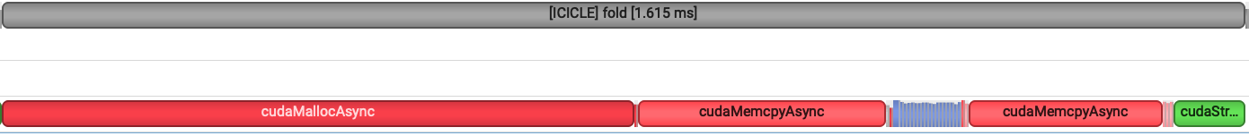
Computation \(\approx 5\%\)

\underbrace{\hspace{322pt}}
\underbrace{\hspace{102pt}}

Memory alloc and copies \(\approx 95\%\)

Profile Analysis: FRI Quotients

\begin{bmatrix} \vdots & \vdots & & \vdots & & \vdots \\[5pt] \textcolor{lightgreen}{f_1(X)} & \textcolor{lightgreen}{f_2(X)} & \dots &\textcolor{lightgreen}{f_i(X)} & \dots & \textcolor{lightgreen}{f_{n_1}(X)} \\[5pt] \vdots & \vdots & & \vdots & & \vdots \end{bmatrix}
\begin{bmatrix} \vdots & \vdots & & \vdots \\[5pt] \vdots & \vdots & & \vdots \\[5pt] \textcolor{red}{f_1(X)} & \textcolor{red}{f_2(X)} & \dots & \textcolor{red}{f_{n_2}(X)} \\[5pt] \vdots & \vdots & & \vdots \\[5pt] \vdots & \vdots & & \vdots \\[5pt] \end{bmatrix}
  • Parallelising across polynomials can give \(\approx2000\times\) speedup
z: \begin{bmatrix} \textcolor{lightgreen}{f_1(z)} & \ \ \textcolor{lightgreen}{f_2(z)} & \ \dots \ & \textcolor{lightgreen}{f_i(z)} & \ \dots \ & \ \textcolor{lightgreen}{f_{n_1}(z)} \end{bmatrix}
zg: \begin{bmatrix} \textcolor{lightgreen}{f_1(zg)} & & & & & & \ \ \textcolor{lightgreen}{f_i(zg)} & & & & & & \ \end{bmatrix}
z: \begin{bmatrix} \textcolor{red}{f_1(z)} & \ \ \textcolor{red}{f_2(z)} & \ \dots \ & \ \textcolor{red}{f_{n_2}(z)} \end{bmatrix}
zg: \begin{bmatrix} & & & \ \textcolor{red}{f_2(zg)} & & & & & & \ \\ \end{bmatrix}
\underbrace{\hspace{397pt}}

Computation and malloc \(\approx 0.34\%\)

\underbrace{\hspace{190pt}}\dots

Memory alloc and copies \(\approx 99\%\)

\(\implies 300\times\) speedup

Profile Analysis: Summary

  • Parallelising across polynomials can give \(\approx2000\times\) speedup
Stage Same backend prove Modified backend prove
OODS sampling 20x 16% 2000x
FRI Quotient 300x 28% 1000x

STWO Prover Report

By Suyash Bagad

STWO Prover Report

  • 138